
What this is
- easyClock is a user-friendly desktop application for analyzing and visualizing data.
- It simplifies the process of handling multiple time series datasets without requiring coding expertise.
- The application integrates various analytical methods and allows for efficient assessment of rhythmicity and group differences.
- easyClock is designed to enhance accessibility and efficiency in research.
Essence
- easyClock streamlines analysis by providing an intuitive interface for processing multiple datasets simultaneously. It incorporates advanced statistical methods to assess rhythmicity and visualize results without the need for programming skills.
Key takeaways
- easyClock enables batch analysis of time series data, allowing users to analyze multiple files concurrently. This feature significantly reduces the time and complexity involved in research.
- The application includes four analytical methods—Cosinor, Cosine-Kendall, Python-JTK, and Harmonic-Cosinor—tailored for various types of rhythmic data. These methods enhance the robustness of rhythmicity detection.
- A re-analysis of a transcriptomic dataset using easyClock identified 272 cycling genes with < 0.05, demonstrating its effectiveness in handling complex omics data and revealing new insights into gene cycling patterns.
Caveats
- The accuracy of results may be influenced by the quality of input data, particularly in the presence of noise or irregularities. Users should ensure data integrity for optimal outcomes.
- While easyClock supports various analysis methods, the choice of method may affect the detection of rhythmicity. Users need to understand the implications of each method for their specific datasets.
Definitions
- circadian rhythm: Biological processes that display an endogenous oscillation of about 24 hours, influencing behaviors such as sleep and feeding.
- BH.Q: Benjamini–Hochberg adjusted p-value, used to control the false discovery rate in multiple hypothesis testing.
Simplified
Background
The circadian clock governs many physiological processes and animal behaviors, ranging from gene expression to activity, sleep, and feeding [1]. Various tools are available to acquire circadian data, such as behavioral monitors [2 –6], as well as omics methods including transcriptomics, proteomics, and metabolomics [7 –9]. Numerous analysis methods can be employed to determine the rhythmicity of these data, including JTK_CYCLE [10], Cosinor analysis [11], or RAIN [12]. However, most of these tools require some coding expertise [10 –15]. Other graphical user interface (GUI) analyzers, such as ClockLab [16] and ShinyR-DAM [17], are either not freely accessible to users or optimized for specific behaviors. Web-based analysis solutions reduce operational difficulties but pose the risk of inadequate maintenance or computational constraints. While recent circadian rhythm analyzers tend to simplify coding operations and optimize GUI design [18], a more efficient and user-friendly tool would facilitate analysis of data collected from high-throughput experiments. To overcome operational barriers and enhance analysis efficiency, a GUI application named "easyClock" was developed to facilitate the local processing of multiple time series sets. The free-to-use easyClock application offers an intuitive interface and efficient, comprehensive mathematical methods, thereby improving user experience in data analysis and presentation within the field of chronobiology.
Results
Data input and preview

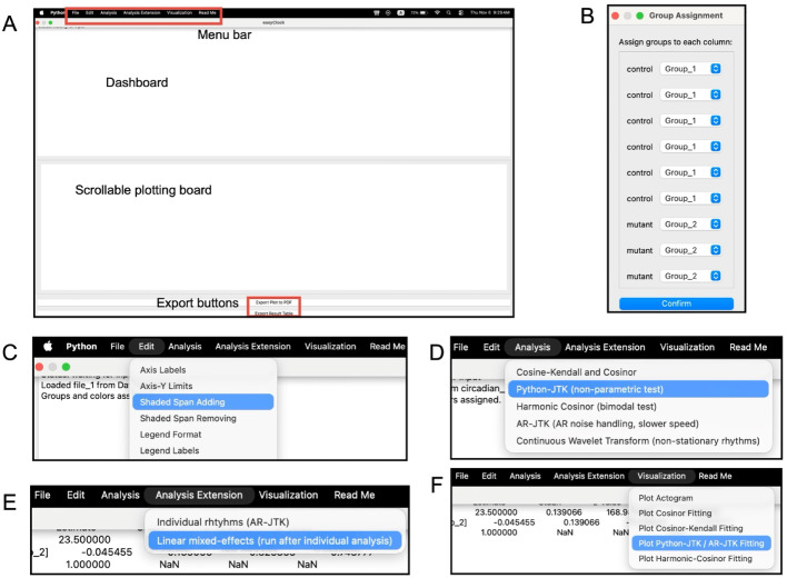
Interface of the easyClock application.The easyClock interface is comprised of four distinct components: a menu bar, a dashboard, a scrollable plotting board, and export buttons. The menu bar, situated at the top of the interface, comprises menus designed to facilitate file input (,), plot editing (), data analysis (,), and visualization () functionalities. Below the menu bar, the dashboard presents a comprehensive display of all execution information and analysis outcomes. The scrollable plotting board serves as a visual representation of the data, offering a preview of all datasets and enabling real-time refreshes through edit capabilities. At the bottom, two buttons are positioned to facilitate the export of plots and analysis results displayed on the boards. The analysis methods typically report four key parameters, including adjustedvalues (ADJ.P or BH.Q), period (PER), amplitude (AMP), and acrophase (peak time) A A B C D E F p

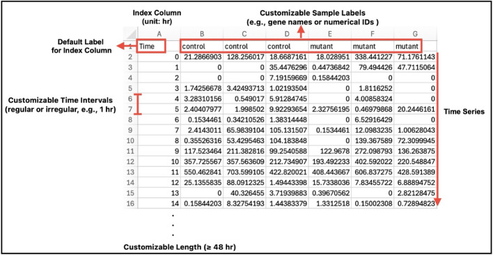
Example of input data format. The easyClock application allows users to load (or cancel) up to three CSV files, each occupying a separate slot. Each file must include an index column with a default label ("Time"), sample labels, and time-series data. The application supports both regular and irregular time intervals. Sample labels should be placed in the first row, starting from the second column, and can be customized as needed. Upon loading, group assignments are automatically generated from the first input file by grouping samples with identical labels; these groupings can be manually adjusted. When analyzing multiple files, groups in subsequent files are assigned automatically based on label matches with the first file. For robust and accurate analyses, at least 48 h of data is recommended, although there is no minimum requirement for data resolution (i.e., the number of data points per sample within a given period)

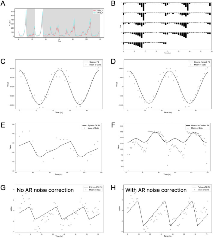
Diverse visualizations in easyClock. easyClock supports the export of various graph types, includingtraditional time-series curves,actograms, andthe best model fits. Representative examples of model fits include:Cosinor,Cosinor–Kendall,Python-JTK, andHarmonic-Cosinor. Panelsandillustrate the effect of the autoregressive noise handling module, shown withoutand withAR noise correction A B C–H C D E F G H G H
Circadian rhythm analysis
Following data input and preview, users can select a file for analysis (Fig. 1D & E). All time-series within the selected file are analyzed, with users prompted to specify the period of interest; a minimum of 48 h is recommended. The current version of easyClock includes four analytical regression methods: Cosinor, Cosine-Kendall, Python-JTK, and Harmonic-Cosinor. To handle autoregressive (AR) noise [19, 20] or non-stationary oscillations [21] often present in real biological data, easyClock also integrates modules that correct for or characterize these effects. Besides, inter-individual variability and group differences can be efficiently assessed using linear mixed-effects modeling [22].
Both the Cosinor and Cosine-Kendall are designed for analyzing cosine-like rhythmic data. In easyClock, the Cosinor method applies ordinary least squares regression to fit a linearized cosine model to the data [11]: \documentclass[12pt]{minimal} \usepackage{amsmath} \usepackage{wasysym} \usepackage{amsfonts} \usepackage{amssymb} \usepackage{amsbsy} \usepackage{mathrsfs} \usepackage{upgreek} \setlength{\oddsidemargin}{-69pt} \begin{document}$$y = M + \beta_{{1}} {\mathrm{cos}}\left( {wx} \right) \, + \, \beta_{{2}} {\mathrm{sin}}\left( {wx} \right) + \varepsilon$$\end{document}. Rhythmicity is assessed using an F-test for the null hypothesis: β1 = β2 = 0. To control for false positives across multiple comparisons within each time series (i.e., across different periods), p-values are adjusted using the Bonferroni correction. The Cosine-Kendall method extends the Cosinor approach by ranking the data to reduce the influence of outliers or non-Gaussian noises. It measures concordance between the ranked input and each ranked cosine reference using the non-parametric test–Kendall's tau rank correlation [23]. The lowest p value from the best-fitting model is selected, and Bonferroni correction is applied for multiple period and lag tests within each time series.
The easyClock package also features a non-parametric test, Python-JTK, which is a modified reimplementation of the original JTK_CYCLE algorithm. Originally developed for R, JTK_CYCLE is widely used for detecting circadian rhythms [10]. It operates by performing rank-based comparisons between the input data and a library of discrete, triangle-shaped templates that may be either symmetric or asymmetric. In easyClock, Python-JTK uses Kendall's tau both to measure similarity and assess statistical significance, bypassing the Jonckheere–Terpstra (JT) test employed in the original algorithm. A key advantage of Python-JTK in easyClock is its ability to automatically accommodate both regular and irregular time intervals, making it suitable for a wide range of experimental designs. To improve computational efficiency, easyClock allows users to customize parameters such as expected period, acrophase, and asymmetry, thereby reducing the number of template comparisons and accelerating the analysis. The Benjamini–Hochberg procedure is applied to adjust raw p-values (reported as BH.Q) when group sizes are large, while the Bonferroni correction is applied within each time series when analyzing smaller group sizes (reported as ADJ.P). To handle the AR noise commonly present in real biological data, easyClock also integrates an AR-JTK module that automatically detects and removes this noise before re-analysis.
Drosophila behaviors, such as sleep and locomotor activity, frequently display bimodal patterns under 12-/12-h light/dark cycles [24]. Traditional unimodal analysis methods are inadequate for capturing these complex rhythms. To address this, easyClock incorporates Harmonic-Cosinor analysis (also known as multiple-component cosinor [25]), which enables the fitting of bimodal waveforms by combining multiple sine and cosine components within each cycle (two components in the current version). The concordance between input data and each composite waveform reference is assessed using Kendall's tau rank correlation, as demonstrated in the Cosinor-Kendall and Python-JTK methods.
| Data types | Rhythmicity | Groups | Period | Amplitude | Nose (amp%) | Asymmetry |
|---|---|---|---|---|---|---|
| Sub-Table : Data simulation 1 | ||||||
| Pseudo-random | NO | 50 | – | – | – | – |
| Cosine | YES | 80 | 24 | 0.001–10000 | 20–40% | NO |
| Triangle | YES | 40 | 24 | 0.015–10000 | 30–40% | YES |
| Bimodal | YES | 32 | 24 | 0.015–10000 | 20% | YES |
| Feature | easyClock | BioDare2 | pyBOAT |
|---|---|---|---|
| Platform | Standalone desktop app (macOS and Windows) | Web-based online service | Python package with GUI |
| Primary focus | Circadian rhythm detection | Circadian rhythm detection | Time–frequency analysis of non-stationary oscillations |
| Accessibility | No limitations; Runs locally | Requires registration; Runs online | No limitations; Runs locally |
| Open source | Yes | No | Yes |
| Computational capacity | Scales with local PC performance | Limited by web server capacity | Scales with local PC performance |
| Data privacy | Local data storage; Full privacy | Require data upload to cloud server | Local data storage; Full privacy |
| Key analytical methods | Harmonic Cosinor, JTK, CWT | JTK, periodogram, Detrending models | CWT, Ridge analysis |
| Group comparisons | Yes, includes LME in v3.0 | Limited to statistical aggregation | Limited to statistical aggregation |
| Data input | Supports multiple files and automatic grouping (customizable by user) | Single file per dataset; grouping must be done manually | Accepts multiple single time series for independent analysis |
| Visualization | Editable and publication-ready plots | Non-editable | Non-editable within GUI |
| Output | Summary tables; Individual statistics; Circadian rhythmicity; Graphs | Summary tables; Individual statistics; Circadian rhythmicity; Graphs | Summary tables; Individual statistics; Graphs |
Visualization
In addition to data preview (Fig. 3A), easyClock enables automatic generation of various graphs (Fig. 1F). Actograms are widely used in circadian rhythm research for visualizing rhythmic patterns and phase shifts in time-series data. Users can quickly export double-plotted actograms (Fig. 3B) for any selected group with a few intuitive clicks, without the need to adjust parameters.
Furthermore, easyClock provides visualization of fitted models following analysis. For each dataset, it displays the best fit of the selected model on the original or group-averaged time series, allowing users to visually assess the quality of rhythmicity detection. Depending on the selected method, users can visualize the fitting results of Cosinor analysis, Cosine-Kendall, Python-JTK, and Harmonic-Cosinor (Fig. 3C–F). Additionally, easyClock can provide visualization of the optimal Python-JTK fit with AR correction (Fig. 3G, H).
easyClock analysis of a transcriptomic dataset
Omics approaches are widely used to screen for cycling genes or proteins, but their scale and complexity pose challenges for rhythmicity analysis. For example, a time-series transcriptome in Drosophila typically comprises thousands of genes, leading to millions of statistical comparisons. To demonstrate how easyClock simplifies these procedures, we re-analyzed a previously published transcriptomic dataset.
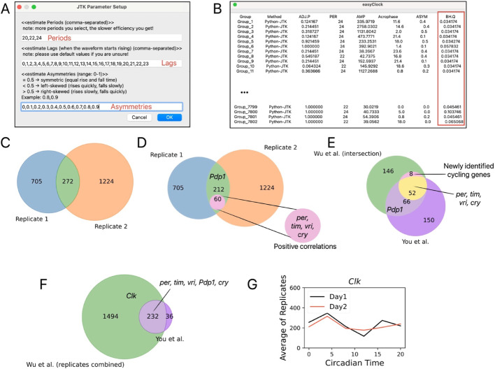
We identified 272 genes with BH.Q < 0.05 in both replicates, including core clock genes such as per, tim, vri, Pdp1, and cry [26, 27] (Fig. 4C). This approach may increase the FDR since replicate-specific noise (e.g., phase-inverted fluctuations) could meet the significance threshold in both replicates without representing reproducible cycling patterns. To address this, we subsequently determined Spearman correlations between replicates for these 272 candidate genes. Sixty genes showed significant positive correlations between replicates (p < 0.05, r > 0), including per, tim, vri, and cry (Fig. 4D). Of these, 52 genes were previously reported as cyclic [7], while 8 genes—including lolal, CG3940, CdsA, alpha-Est10, Ost48, Dh44-R2, CG11241, CG30493—were newly identified and displayed weak cycling patterns (Fig. 4E; Supplementary Fig. 1).
Previous studies combined the replicates for analysis [7], differing from our hybrid approach (intersection + correlation). Nonetheless, easyClock supports both independent and grouped replicate workflows; grouping reduces analysis time but increases file loading duration. Using grouped replicates in easyClock, we identified 1,726 genes with BH.Q < 0.05. Among the 268 previously recognized cycling genes [7], 232 were detected in our grouped analysis, including per,tim, vri, Pdp1, and cry. The Clk gene was newly detected with easyClock in the grouped analysis (Fig. 4F), highlighting the tool's high sensitivity for detecting low-amplitude cycling patterns (Fig. 4G). Overall, easyClock offers an efficient, user-friendly platform for rapid analysis of time-series omics data.
![easyClock analysis of atranscriptome.Key parameters for Python-JTK circadian analysis.Dashboard summary of Python-JTK outputs for 7,802 genes per replicate, with Benjamini–Hochberg-adjustedvalues (BH.Q) highlighted.Venn diagram showing genes with BH.Q < 0.05. The overlap represents 272 genes that cycle in both replicates.Venn diagram highlighting 60 positively correlating genes within the 272-gene overlapping set.Overlap between easyClock cycling genes (272 from both replicates) and previously reported cycling genes from You et al. (268 genes) []. Of these, 52 of the 60 positively correlated genes between replicates were also previously identified as cyclic [].An additional 8 cycling genes, including, were newly identified with the hybrid approach (intersection + correlation).Overlap between genes identified as cyclic by grouped-replicate analysis in easyClock (1,726 genes) and You et al. (268 genes) [], with 232 genes overlapping.Relative expression levels ofacross two days using the averaged values of replicates. All expression data are from the transcriptomic dataset of You et al. [] Drosophila p lolal Clk A B C D E F G [7] [7] [7] [7]](https://europepmc.org/articles/PMC12797594/bin/12859_2025_6340_Fig4_HTML.jpg "Click to view full size")
easyClock analysis of atranscriptome.Key parameters for Python-JTK circadian analysis.Dashboard summary of Python-JTK outputs for 7,802 genes per replicate, with Benjamini–Hochberg-adjustedvalues (BH.Q) highlighted.Venn diagram showing genes with BH.Q < 0.05. The overlap represents 272 genes that cycle in both replicates.Venn diagram highlighting 60 positively correlating genes within the 272-gene overlapping set.Overlap between easyClock cycling genes (272 from both replicates) and previously reported cycling genes from You et al. (268 genes) []. Of these, 52 of the 60 positively correlated genes between replicates were also previously identified as cyclic [].An additional 8 cycling genes, including, were newly identified with the hybrid approach (intersection + correlation).Overlap between genes identified as cyclic by grouped-replicate analysis in easyClock (1,726 genes) and You et al. (268 genes) [], with 232 genes overlapping.Relative expression levels ofacross two days using the averaged values of replicates. All expression data are from the transcriptomic dataset of You et al. [] Drosophila p lolal Clk A B C D E F G [7] [7] [7] [7]
Conclusions
Over the past several decades, various analytical and statistical methods have been developed and adopted in chronobiology, ranging from visual inspection of actograms to sophisticated mathematical statistics [28]. Among these, Analysis of Variance (ANOVA) has served as a fundamental tool for detecting the oscillatory characteristics of circadian data. However, ANOVA alone cannot directly demonstrate the presence of rhythmicity. To overcome this limitation, model-fitting techniques have been introduced. In response to the need for a versatile, accessible, and user-friendly circadian analysis toolkit, we developed easyClock—a GUI application that integrates comprehensive fitting models for circadian rhythm detection. Compared to other tools such as Python packages with GUIs (e.g., pyBOAT [29]) or web-based analyzers (e.g., BioDare2 [30]), easyClock not only integrates their advantages but also implements specific modules that are particularly helpful for chronobiologists, including noise handling, group comparisons, and editable visualizations (Table 2).
In easyClock, amplitude serves as a primary measure of rhythmic strength—a key concept in chronobiology that distinguishes robust circadian patterns from weak or noisy signals. Weak rhythms are typically characterized by irregular peaks, inconsistent phases, or diminished amplitudes. In addition to amplitude-based assessments, the chi-square periodogram (CSP) is commonly employed to quantify rhythmic strength by evaluating deviations from the global mean at each circadian time point [31]. Although high CSP values generally indicate strong rhythmicity, this method can be susceptible to false positives in the presence of substantial fluctuations within the time series [32]. As an extensible platform, future updates of easyClock intend to integrate more comprehensive and reliable methods for assessing rhythmic strength.
Supplementary Information
Below is the link to the electronic supplementary material.
Supplementary Material 1